Economies of Quality - Levelized Cost on Long Time Horizons

Modern economies tend to organize themselves to produce larger volumes of lower-quality goods. This results in lower initial capital expenditures (CAPEX) unlocking greater sales for the seller but at the expense of higher operational expenditures (OPEX) for the buyer, including replacement costs, resulting in higher levelized cost (LC) of goods. This applies to everyday consumer goods like coffee machines, furniture, and homes; as well as industrial systems like power-generating equipment and infrastructure. We provide a simple model to estimate the LC by introducing the idea of economies of quality which defines OPEX as a function of CAPEX with a scaling exponent ($\alpha$). When the scaling exponent exceeds one and for many financial conditions, we find that non-zero CAPEX can minimize long-term cost. This finding is consistent with the everyday notion that spending on higher quality is worth it. Overall we suggest that prioritizing higher CAPEX is economically advantageous under many conditions challenging the dominant CAPEX-minimization strategies rooted in seller-side profit-seeking and buyer-side short-termism.

Introduction

A good has a capital expenditure (CAPEX) and operational expenditure (OPEX). The producer of goods typically chooses a lower upfront CAPEX for himself in exchange for higher OPEX for the customer. The CAPEX takes place at the beginning of the project, and lowering CAPEX often enables the sale. The OPEX occurs annually over the project's lifetime and is often less visible to the customer. A large part of the OPEX is the maintenance and eventual replacement of the CAPEX. If service is required for 100 years but the system only has a lifetime of 50 years, it will have to be replaced at the 50-year mark, which constitutes an OPEX.

Larger CAPEX can reduce the OPEX over the lifetime through various means. Consider a 1950s refrigerator built like a tank with simple components and massive performance margins on the parts. For example, the frame may be built out of stainless steel of considerable thickness and oversized attachment areas; plastic parts are limited or excluded; the parts are bulky and large. The refrigerator is likely to still function today with original components and may require the occasional modular fix or coolant replenishment. Compare that to a modern refrigerator made entirely of unique injection-molded plastics where the margin has been whittled to zero, and the whole thing is designed for planned obsolescence, with myriad single points of failure.

Similarly, consider a home made of brick or stone, with wood or tile flooring, and high ceilings. This home could well last 300 to 1000 years, as can be seen in many historic districts of Europe, and perhaps indefinitely because the engineering margins allow it to do so and because the initial investment in quality ensures it remains a coveted and high-value asset. Now compare that to a stick-built house made of plywood and whittled 2x4s with low ceilings and linoleum floors. The stick-built house has a lifetime of 30-60 years. For the stick-built house, upfront CAPEX is reduced by lowering quality, margins, and material. This leads to an overall reduction in the lifetime and ensures its eventual demolition, overall leading to a higher OPEX to replace components and eventually the entire system.

Producers greatly prefer the modern refrigerator and the stick-built house as they unlock larger volumes and perpetual sales, and today, most houses, buildings, and factories are constructed in this fashion. Companies that opt for quality and long-lived products cannot hope to compete with the short-termist producers because the revenues and market share are not comparable. The rare cases where extreme quality and long-life is unavoidable often lead to stagnant companies that saturate the market. One example could be Bialletti, the makers of the Moka coffee pot which is effectively indestructible, thus limiting the company's long-term growth.

While the reduced upfront CAPEX will expand the market and produce more total refrigerators or houses, the OPEX is higher for the customer. In many cases, the customers suffer from short-termism, choosing short-term gains at a long-term loss. We can analyze this situation to show in what cases a higher upfront CAPEX will lower the overall levelized cost.

Analysis

Assuming self-financed CAPEX in the first year, which is equivalent to the debt or equity financing case, and operations starting after the first year and up to the $N$th year, the levelized cost is given by the below equation for $N$ years of service, $C_0$ the CAPEX, and $c_1$ the yearly OPEX. Note that the cash flows are both discounted (nominal interest rate $i$) and inflated (expected inflation rate $\pi_e$) [1].

$$LC(C_0) = \frac{C_0 + \sum_{n=1}^{N} c_1 \frac{(1+\pi_e)^n}{(1+i)^n}}{\sum_{n=1}^{N} Q \frac{(1+\pi_e)^n}{(1+i)^n}}$$

The main assumption of this analysis is the below expression for the operating cost where we introduce the idea of economies of quality. We consider that $c_1$ is composed of two parts: one is a function of the CAPEX and other ($A$) defines other operations costs such as refueling, labor, or cleaning. The second term is the CAPEX replacement cost per unit time, obtained by dividing the total CAPEX by $t$ which can be considered the system lifetime or replacement time.

$$c_1 = f(C_0) = A + \frac{C_0}{t}$$

The replacement time is a function of the CAPEX, with subscript $R$ representing a reference point. The exponent $\alpha$ used to obtain the replacement time is a scaling exponent on the normalized cost. It can be thought of as economies of quality.

$$t(C_0) = t_R \left(\frac{C_0}{C_R}\right)^\alpha$$

For many components, a cost and performance metric like this will be sublinear ( $0 < \alpha < 1$) or simply take on a fixed value ( $\alpha = 0$ ). This is the case for luxury or military goods where spending 10x more will barely nudge a given performance or utility metric. However, $t\left(C_0\right)$, the lifetime, can often be a linear or higher power relation with respect to the capital cost factor. The linear case can be considered as simple margin or redundancy. We can double the lifetime of a component by doubling the margin on the lifetime-limiting parameter. We can also add the same component to the initial inventory for a simple swap-in the future. A case for high economies of quality could be, for example, a brick or stone house which may have 1-3x higher upfront CAPEX but a 5-10x longer replacement lifetime which is described by $\alpha \sim 2$. Data, should it exist, is not reviewed here.

Now to estimate the LC and LC-minimizing case, we make the necessary substitutions. We define the net present value factor $\beta$ which is the sum of the NPVs of a constant cashflow that is both inflated and discounted.

$$\beta(\pi_e,i) = \sum_{n=1}^{N} \frac{(1+\pi_e)^n}{(1+i)^n}$$

We define the variable $r$ as the ratio of the inflation to the interest rate.

$$r = \frac{1+\pi_e}{1+i}$$

Note that $r$ is related to the real interest rate $r_{real}$ as below. Historically, $r$ is less than 1 as interest rates should incentivize a return better than inflation. Over the period 1984 to 2024, the US 10-year real interest rate averages to 2.25%, corresponding to $r$ of 0.978 [0].

$$1+r_{real} = \frac{1}{r}$$

The net present value factor is a geometric series and can be simplified as follows.

$$\beta(r) = \sum_{n=1}^{N} r^n = \frac{r(r^N-1)}{r-1}$$

Substituting $\beta$ into the LC:

$$LC(C_0) = \frac{C_0 + \beta c_1}{Q\beta} = \frac{C_0}{Q\beta} + \frac{c_1}{Q}$$

Substituting $c_1$ and the replacement time $t$:

$$LC(C_0) = \frac{1}{Q} \left( \frac{C_0}{\beta} + A + \frac{C_R^\alpha C_0^{1-\alpha}}{t_R} \right)$$

And minimizing $LC$ yields the following optimal CAPEX:

$$\frac{C_{0, \min}} {C_R} = \left(\frac{\beta (\alpha - 1)}{t_R }\right)^{1/\alpha} = \left(\frac{\frac{r(r^N-1) }{r-1}(\alpha - 1)}{t_R }\right)^{1/\alpha}$$

This function has an interesting shape. It exists only for $\alpha > 1$, and it is always positive with a peak $\alpha$. Looking at the derivative

$$\frac{d}{d\alpha} \left( \left( A (\alpha - 1) \right)^{\frac{1}{\alpha}} \right) = \frac{\left( A (\alpha - 1) \right)^{\frac{1}{\alpha}} \left( \frac{\alpha}{\alpha - 1} - \log \left( A (\alpha - 1) \right) \right)}{\alpha^2}$$

We are met with a transcendental equation. In any case there is a cost optimizing quality that is neither 0 nor infinite.

$$\frac{\alpha}{\alpha - 1} = \log \left( A (\alpha - 1) \right)$$

Results

We have parameterized the LC with a few coefficients and exponents to include the effects of maintenance and replacement as a function of CAPEX, and finally showed the existence of optimal CAPEX greater than 0 for $\alpha > 1$ under certain conditions. Those OPEX costs not related to CAPEX are contained in the constant $A$ and have no effect on the LC-minimizing CAPEX but can reduce the importance of the optimal CAPEX.

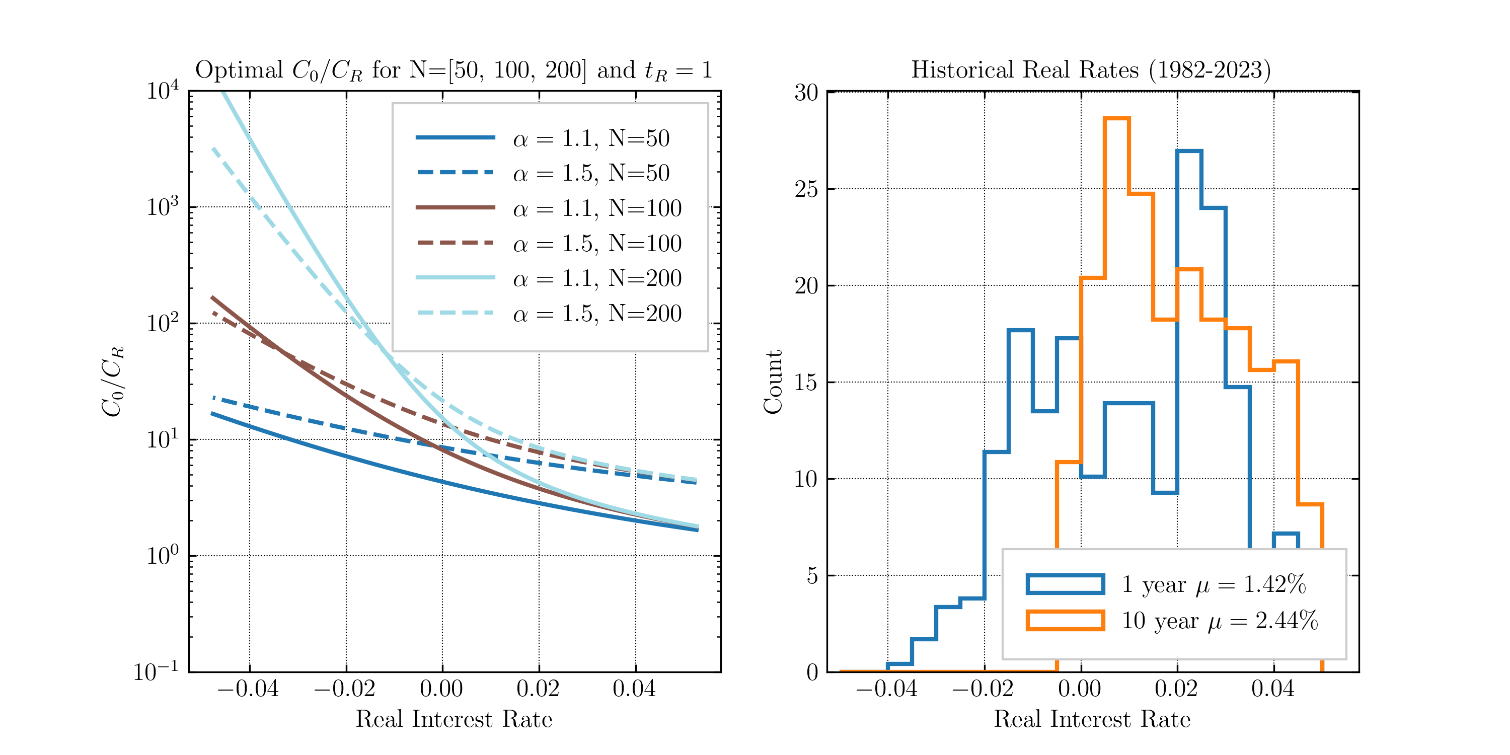
We visualize, in Figure 1, the LC-minimizing $C_{0,\ \min}$ across real interest rates and for different $\alpha$, the economies of quality, and $N$, the project lifetime. The particular example here utilizes a reference replacement time $t_R$ of 1 year. Increasing $t_R$ will shift the lines down. The LC-minimizing CAPEX is higher for larger $\alpha$, longer project lifetimes, and lower real interest rates. When $\alpha < 1$, CAPEX should be minimized to minimize the LC.

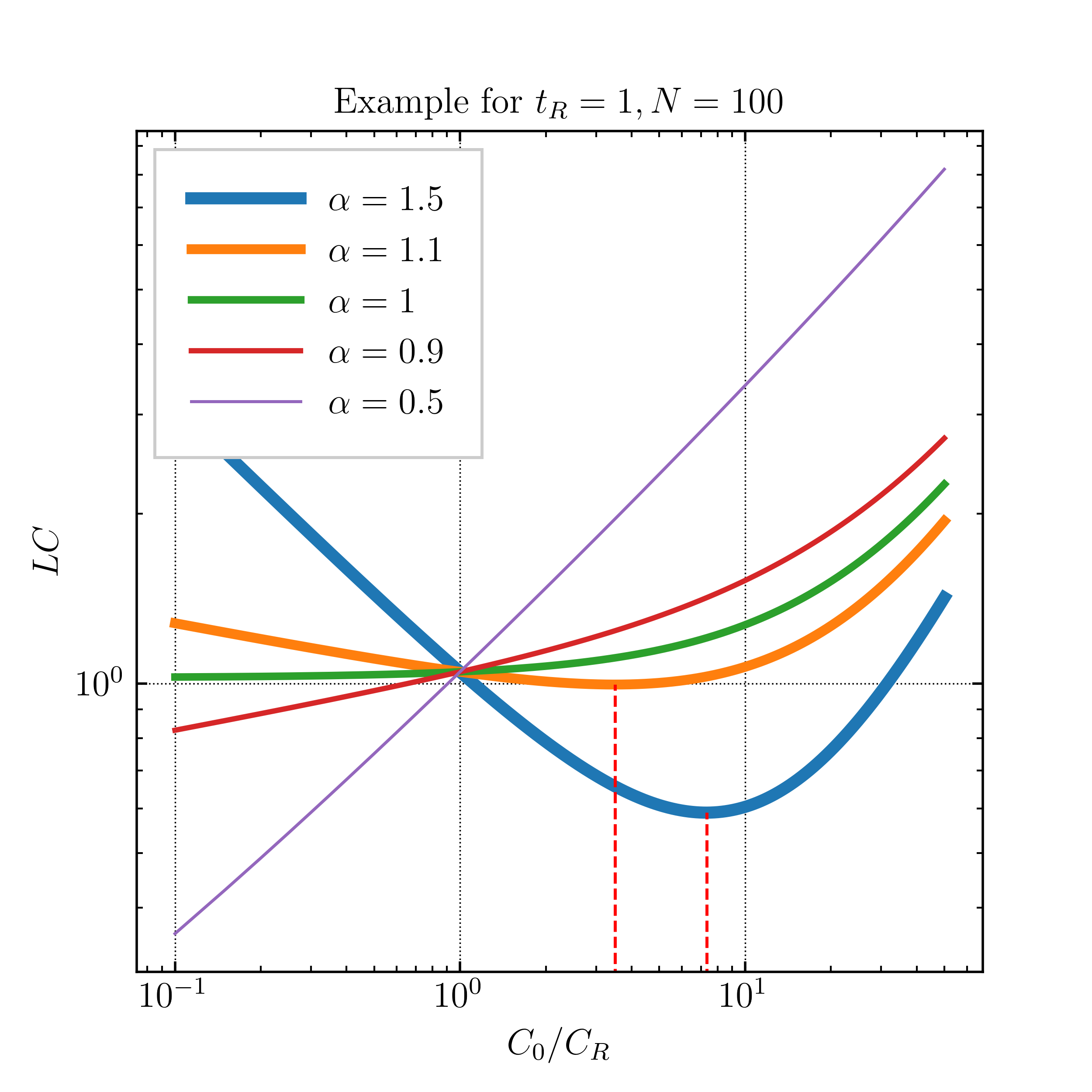
In Figure 2, we show the LC or value versus the relative CAPEX under different inflation and discount rates for a 100-year project. LC is estimated as the net present value of the costs over the net present value of production, measured in years. Cashflows are inflated and discounted to the net present value assuming the indicated inflation and discount rate. The reference cost and replacement time, $[C_R, t_R]$, are set to [1, 1], and $A$ is set to 0.05. Each line corresponds to a different $\alpha$, going from 0.5 to 1.5. $\alpha$ represents diminishing extension of lifetime on additional CAPEX. This shows a clear example of the ways to minimize the LC in different conditions.

Figure 1 Left: optimal CAPEX relative to reference vs real interest rate. Lines for 𝑁, the project lifetime, and 𝛼, the economies of quality. Right: histogram of historical US real interest rates

Figure 2 Levelized cost for 100 year project lifetime at the historically average real interest rate of 2.25%. Red dashed lines indicate the non-zero minima. 𝛼 determines the scaling for OPEX as a function of CAPEX.

Conclusions

Many projects utilize imprecise and hand-wavy estimates on the operational costs and project lifetime, as these quantities involve future predictions both of the system's performance and financial conditions. Most projects are evaluated with a large focus on the CAPEX, a near-term and more clearly predictable cash flow. In this way, CAPEX is often blindly minimized without finding the balance between CAPEX and OPEX that would minimize LC. This is done most egregiously with projects with new technologies where the replacement time, project lifetime, and operational costs are not well known.

OPEX is basically ignored for consumer goods as the consumer will not typically bother with a lifetime cost estimate, or at best, will shortchange himself by thinking only in the short term and for himself rather than the many generations to come. Similarly, OPEX and replacement costs are underutilized in architecture and buildings. It must be said that estimating lifetime and replacement times is quite difficult, as it involves not only the durability of the system but also the motions of culture and technology that may in the future decide that the project is ugly or inefficient and worthy of demolition. The evaluation of engineered systems and goods like buildings and cars should include a price for having to look at them. A cost-minimized monstrosity is still a monstrosity, and this often determines the lifetime of a project, for we typically only conserve beautiful things. So despite the difficulty, we should attempt to estimate these OPEX costs.

Both producers and consumers are predisposed to prefer low CAPEX rather than a lower LC because of profit-seeking, short-termism, and a general inability to predict and reason about LC. Further exacerbating these trends are high interest rates, which are, in many circles, considered a deformity and injustice of the fiat monetary system and government-backed currencies, as they lower the LC-minimizing CAPEX. All this yields non-optimal LC, market inefficiencies, and ultimately the waste of resources and opportunities to make long-lasting and beautiful things.

This analysis introduced the idea of economies of quality to relate the OPEX to the CAPEX using the replacement time. This relation requires a reference point for CAPEX and replacement time. It uses a scaling law with an adjustable parameter that can be determined using data, although we did not undertake that exercise. With this assumption, LC can be estimated and there exist cases in which LC is minimized by non-zero CAPEX.

Questions remain regarding the validity of the economies of quality, the specific exponents to use, and what assumptions should be made on interest rates which vary so widely and senselessly over time. Another consideration is the effect of technological development. While many projects have historically been perennial, especially those that must satisfy human needs with examples in furniture, buildings, roads, and even power, etc., it is not clear what the phenomenon of accelerating technological development will mean for project obviation. It would be silly to design a 500-year power plant with technology that will be obsolete in less than 50 years, but certain aspects may be perennial such as the civil works, heat rejection, and grid interconnections. In our everyday lives, it seems like there can be long-lasting artifacts that withstand generations, whose essence is true and good and transcends fashions and whims.

[1] Harvey, L. D. (2020). “Clarifications of and improvements to the equations used to calculate the levelized cost of electricity (LCOE), and comments on the weighted average cost of capital (WACC).” Energy, 207, 118340.

[2] Federal Reserve Bank of St. Louis (2024). “Real interest rate: 10-year treasury rate minus expected inflation, https://fred.stlouisfed.org. Type: REAINTRATREARAT10Y, Accessed: 2024-05- 26.